using GMT
GMT.resetGMT() # hide
G = earthtide(T="2022-07-07T12:00:00");
imshow(G, coast=true, colorbar=true, title="Earth tide at noon 7-July-2022")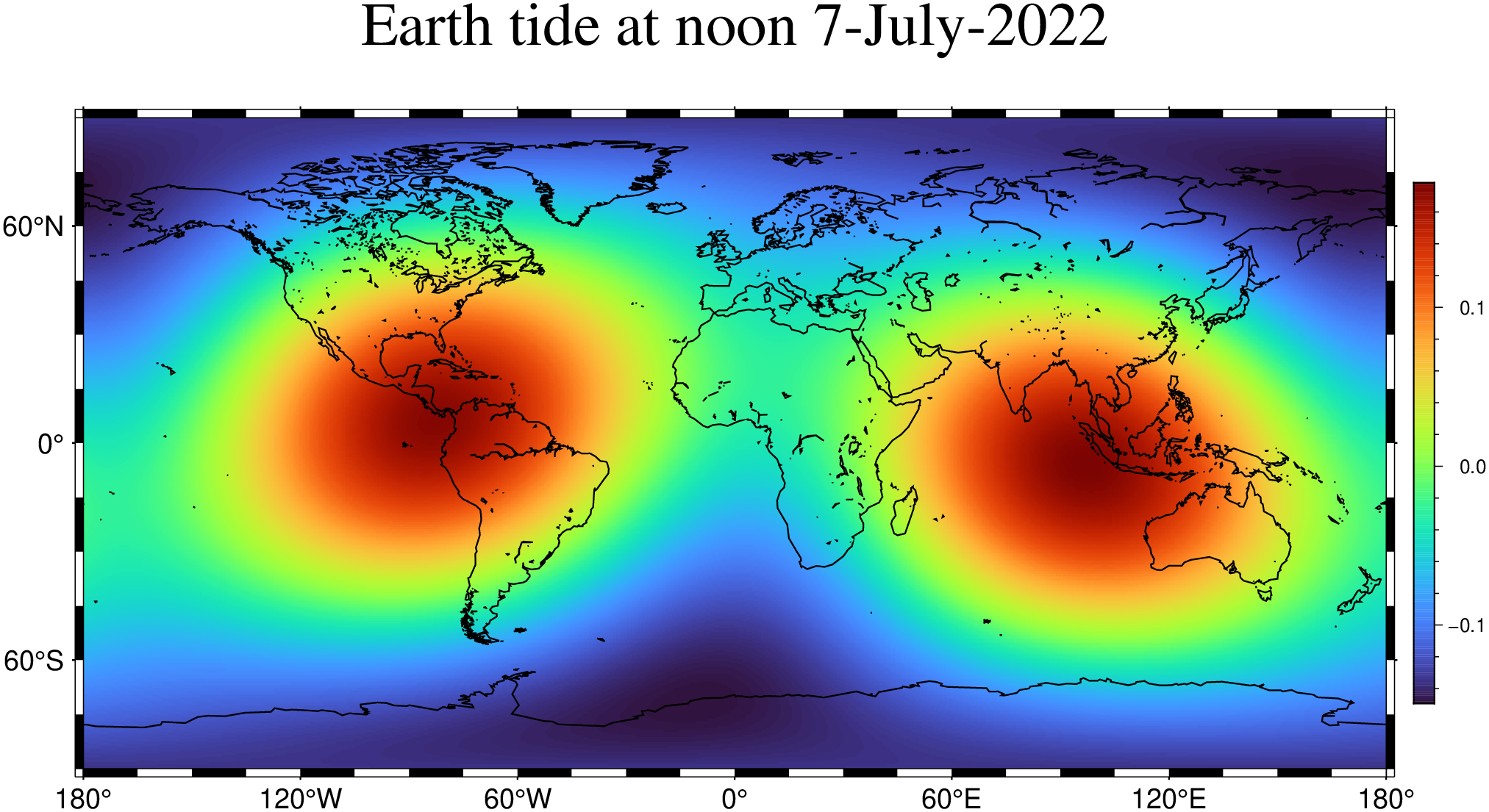
Did you know that it’s not only the oceans that have a tide? Yes, the solid Earth has tides as well, and they are not so small as one might imagine.
This example shows a global view of the vertical component of the Earth tide for a perticular data.
using GMT
GMT.resetGMT() # hide
G = earthtide(T="2022-07-07T12:00:00");
imshow(G, coast=true, colorbar=true, title="Earth tide at noon 7-July-2022")
Now we show the three components of the Earth tide for a specific location (the Panama Cannal) and time interval (the 7’th July 2022).
First we compute the components that will come out in a with named columns. This is handy because we can refer to them by name instead of by column number.
using GMT, PrettyTables   # hide
getpath4docs(file::String) = joinpath("..", "..", "..", "..", "..", file) # hide
io = IOBuffer() # hide
D = earthtide(range=("2022-07-07T", "2022-07-08T", "1m"), location=(-82,9))
PrettyTables.pretty_table(io, D.data[1:5,:]; header=D.colnames, backend=Val(:html)) # hide
println("~~~" * String(take!(io)) * "~~~") # hide
Now plot the three of them with a legend
using GMT
D = earthtide(range="2022-07-07T/2022-07-08T/1m", location=(-82,9));    # hide
plot(D[:Time, :Vertical], lc=:red, lw=1, legend=:Vertical,
     title="Earth tide components (m) at Panama Cannal")
plot!(D[:Time, :East],  lc=:green, lw=1, legend=:East)
plot!(D[:Time, :North], lc=:blue,  lw=1, legend=:North, show=true)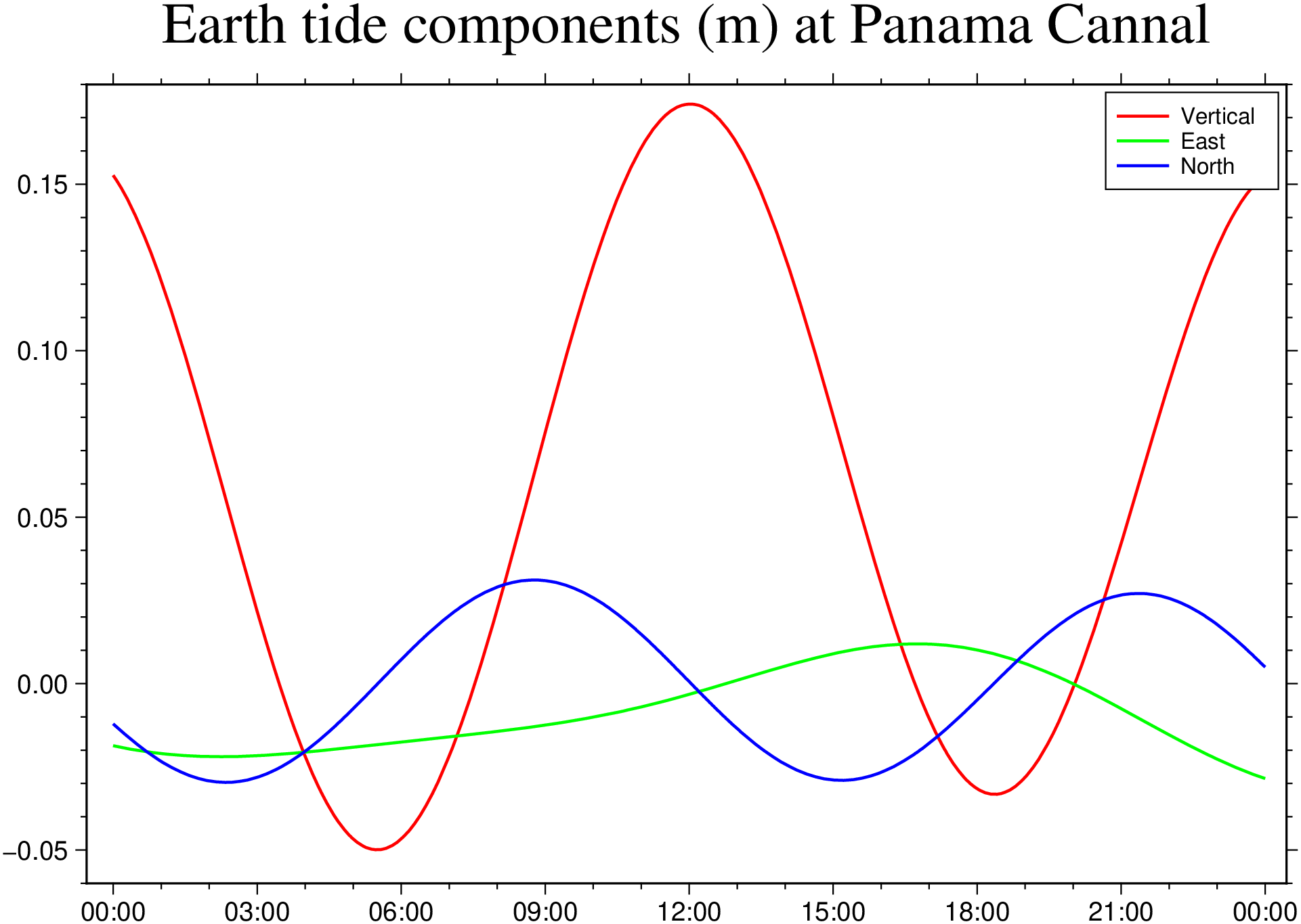
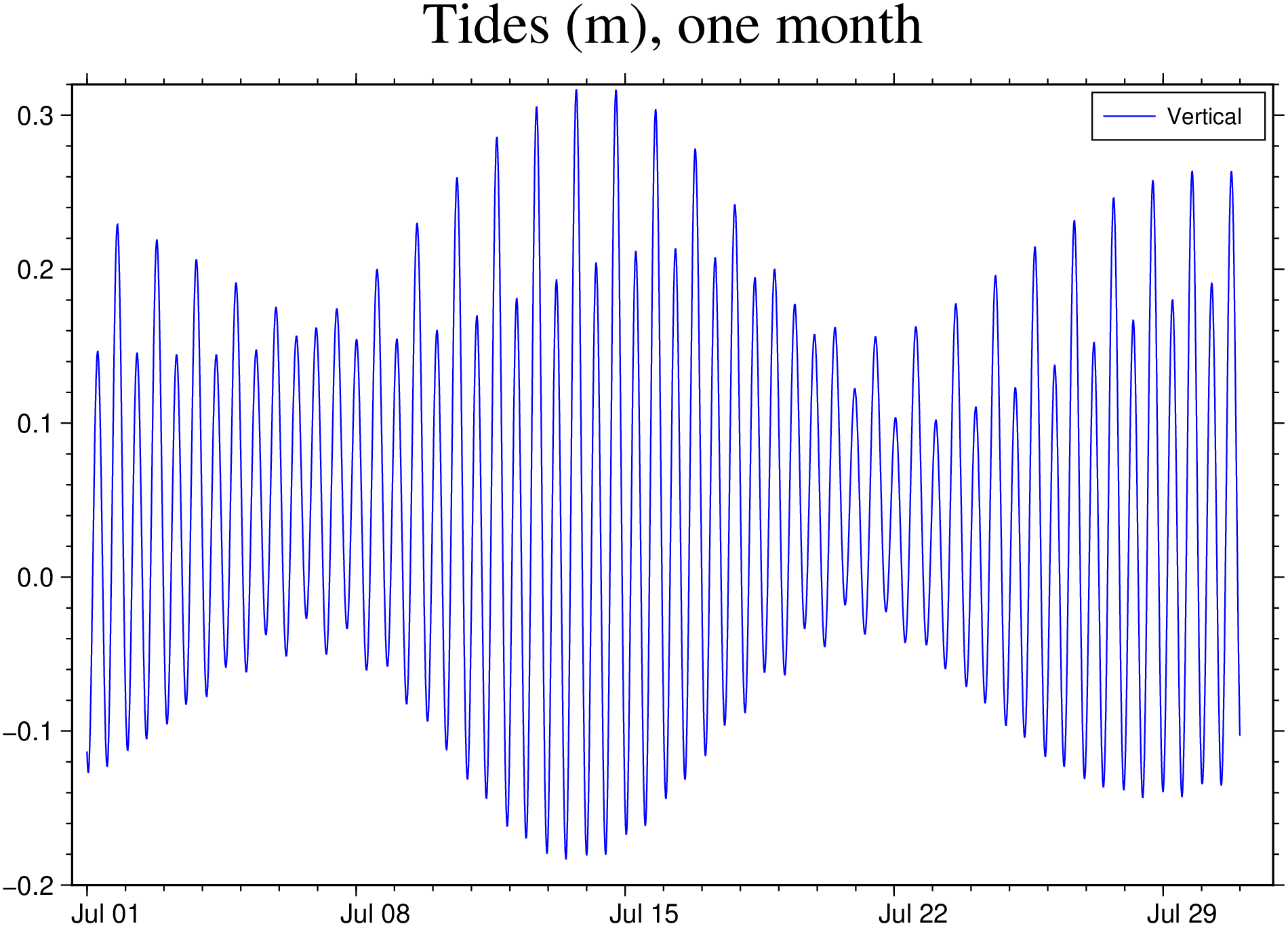
And now, let’s see a full month of tidal data (vertical component).
using GMT
D = earthtide(range=("2022-07-01T", "2022-07-31T", "1m"), location=(-82,9));
plot(D[:Time, :Vertical], lc=:blue, legend=:Vertical, title="Tides (m), one month", show=true)